1. Open MATLAB. Open the editor and copy paste the following code. Name your code as FirstCode.m
Save the resulting plot as a JPEG image and put it here:
clear all;
close all;
x = [1 2 3 4 5];
y = 2.^x;
plot(x, y, 'LineWidth', 6);
xlabel('Numbers', 'FontSize', 12);
ylabel('Results', 'FontSize', 12);
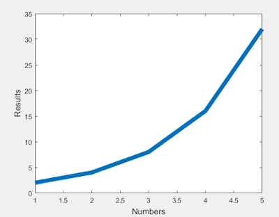 |
| Figure 1: Shows the exponentially generated line created in MATLAB |
2. What does clear all do?
- Clear all clears all of the previous commands that are left in the command window.
3. What does close all do?
- Closes all of the figures and windows that have been made previous to this command.
4. In the command line, type x and press enter. This is a matrix. How many rows and columns are there in the matrix?
- This matrix has 5 columns and 1 row.
5. Why is there a semicolon at the end of the line of x and y?
- This semicolon prevents the command from showing up in the command window, but still allows the command to go through. The semi-colon is there to end the variable's statement.
6. Remove the dot on the y = 2.^x; line and execute the code again. What does the error message mean?
- The period is there to allow multiplication with a matrix (or multiple values) 'x' is a matrix.
7. How does the LineWidth affect the plot? Explain.
- Line Width makes allows you to change the thickness of the graph.
8. Type help plot on the command line and study the options for plot command. Provide how you would change the line for plot command to obtain the following figure (Hint: Like ‘LineWidth’, there is another property called ‘MarkerSize’)
clear all;
close all;
x = [1 2 3 4 5];
y = 2.^x;
plot(x, y,'ro-', 'LineWidth', 6, 'markersize', 20)
xlabel('Numbers', 'FontSize', 12)
ylabel('Results', 'FontSize', 12)
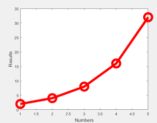 |
| Figure 2: Same as the first figure but with the added feature called 'markersize'. |
9. What happens if you change the line for x to x = [1; 2; 3; 4; 5]; ? Explain.
- This adjusts the matrix by making it have 1 column and 5 rows. The semi columns cause you to "enter" within the matrix, moving your next entry down a row.
10. Provide the code for the following figure. You need to figure out the function for y. Notice there are grids on the plot.
clear all;
close all;
x = [1 2 3 4 5];
y = x.^2;
plot(x, y, 'sk:', 'LineWidth', 6, 'markersize', 20);
xlabel('Numbers', 'FontSize', 12);
ylabel('Results', 'FontSize', 12);
grid on;
set(gca, 'gridlinestyle', ':')
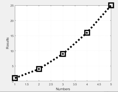 |
| Figure 3: Shows the replicated plot, with the 'y' function and grids. |
(a.) Calculate sinus of 30 degrees using a calculator or internet.
- sin(30) = 0.5
(b.) Type sin(30) in the command line of the MATLAB. Why is this number different? (Hint: MATLAB treats angles as radians).
--------------------------------------------------------------------------------------------------------------------------
>> sin(30)
ans =
-0.9880
--------------------------------------------------------------------------------------------------------------------------
- This number is different because 30 radians is not equivalent to 30 degrees and Matlab is doing the calculation with respect to radians while my calculator is doing the calculation with respect to degrees.
(c.) How can you modify sin(30) so we get the correct number?
- The command "sind( )" allows you to evaluate the problem with respect to degrees instead of radians.
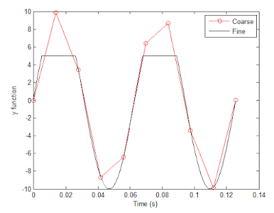
12. Plot y = 10 sin (100 t) using MATLAB with two different resolutions on the same plot: 10 points per period and 1000 points per period. The plot needs to show only two periods. Commands you might need to use are linespace, plot, hold on, legend, xlabel, and ylabel. Provide your code and resulting figure. The output figure should look like the following:
clear all;
close all;
clc;
x = linspace(0, 0.1256636,10);
y = 100*sin(100*x);
plot(x, y, 'ro-');
hold on;
z = linspace(0, 0.1256636,2000);
q = 100*sin(100*z);
plot(z, q);
xlabel('Time (s)');
ylabel('y function');
legend('Coarse', 'Fine');
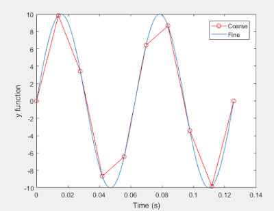 |
| Figure 4: Replicated figure, two resolutions of y = 10*sin(100*t) are plotted. |
- The difference between the plot and the one in figure 4 is that in this one the "Fine" line is capped off with a maximum of 5.
clear all;
close all;
clc;
x = linspace(0, 0.1256636, 10);
x1 = linspace(0, 0.1256636, 2000);
y = 10*sin(100*x);
plot(x, y, 'ro-');
hold on;
y1 = 10*sin(100*x1);
z = find(y1 > 5);
y1(z) = 5;
plot(x1, y1, 'k');
xlabel('Time (s)');
ylabel('y function');
legend('Coarse', 'Fine');
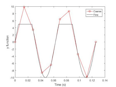 |
Figure 5: is our attempt at replicating the plot from the
previous question
|
PART B: Filters and MATLAB
1. Build a low pass filter using a resistor and capacitor in which the cut off frequency is 1 kHz. Observe the output signal using the oscilloscope. Collect several data points particularly around the cut off frequency. Provide your data in a table.
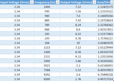 |
| Table 1: Data collected from a Low Pass circuit. |
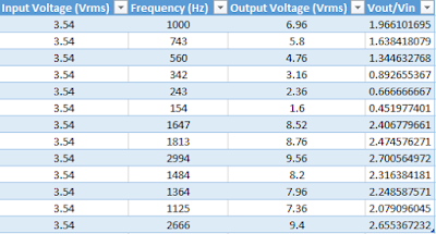 |
| Table 2: Data Collected from a High Pass circuit. |
2. Plot your data using MATLAB. Make sure to use proper labels for the plot and make your plot line and fonts readable. Provide your code and the plot.
clear all;
close all;
x = [1000 990 980 889 789 688 589 299 104 1113 1300 2331 3000 5023 7588 4242 6500];
y = [2.124 2.1356 2.1469 2.237 2.3277 2.4294 2.5198 2.7571 2.825 2.011 1.853 1.22 0.983 0.621 0.429 0.734 0.497];
X = sort(x);
Y = sort(y, 'descend');
plot(X, Y, '-ro', 'MarkerSize', 5);
xlabel('Frequency', 'FontSize', 12);
ylabel('Vout / Vin RMS', 'FontSize', 12);
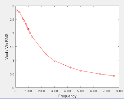 |
| Figure 6: Data from Low Pass circuit (Table 1) plotted in MATLAB. |
clear all;
close all;
x = [1000 743 560 342 243 154 1647 1813 2994 1484 1364 1125 2666];
y = [1.966 1.638 1.344 0.892 0.666 0.4519 2.406 2.474 2.700 2.316 2.248 2.079 2.655];
X = sort(x);
Y = sort(y);
plot(X, Y, '-ro', 'MarkerSize', 5);
xlabel('Frequency', 'FontSize', 12);
ylabel('Vout / Vin RMS', 'FontSize', 12);
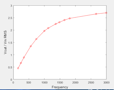 |
| Figure 7: Data from High Pass circuit (Table 2) plotted in MATLAB. |
clear all;
close all;
x = [1000 990 980 889 789 688 589 299 104 1113 1300 2331 3000 5023 7588 4242 6500];
y = [2.124 2.1356 2.1469 2.237 2.3277 2.4294 2.5198 2.7571 2.825 2.011 1.853 1.22 0.983 0.621 0.429 0.734 0.497];
X = sort(x);
Y = sort(y,'descend');
plot(X, Y,'r', 'LineWidth', 6)
xlabel('Frequency (kHz)', 'Fontsize', 12)
ylabel('Amplitude of Vout (V)', 'FontSize', 12)
hold on;
k = find (Y > 5.96 * 0.65, 1, 'last');
X(k)
4. Put a horizontal dashed line on the previous plot that passes through the cutoff frequency.
clear all;
close all;
x = [1000 990 980 889 789 688 589 299 104 1113 1300 2331 3000 5023 7588 4242 6500];
y = [2.124 2.1356 2.1469 2.237 2.3277 2.4294 2.5198 2.7571 2.825 2.011 1.853 1.22 0.983 0.621 0.429 0.734 0.497];
X = sort(x);
Y = sort(y,'descend');
plot(X, Y,'r', 'LineWidth', 6);
xlabel('Frequency (kHz)', 'Fontsize', 12);
ylabel('Amplitude of Vout (V)', 'FontSize', 12);
hold on;
x1 = (0:7588);
y1 = 0.707*2.825;
plot(x1, y1,'b+', 'LineWidth', 2);
xlabel('Frequency (kHz)', 'Fontsize', 12);
ylabel('Amplitude of Vout (V)', 'FontSize', 12);
hold off;
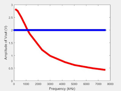 |
| Figure 8: Low Pass filter circuit's data plotted with cutoff frequency line |
5. Repeat 1-3 by modifying the circuit to a high pass filter.
clear all;
close all;
x = [1000 743 560 342 243 154 1647 1813 2994 1484 1364 1125 2666];
y = [1.966 1.638 1.344 0.892 0.6666 0.4519 2.406 2.4745 2.700 2.316 2.248 2.079 2.655 ];
X = sort(x);
Y = sort(y);
plot(X, Y,'r', 'LineWidth', 6);
xlabel('Frequency (kHz)', 'Fontsize', 12);
ylabel('Amplitude of Vout (V)', 'FontSize', 12);
hold on;
x1 = (0:2994);
y1 = 0.707*2.700;
plot(x1, y1,'b+', 'LineWidth', 2);
xlabel('Frequency (kHz)', 'Fontsize', 12);
ylabel('Amplitude of Vout (V)', 'FontSize', 12);
hold off;
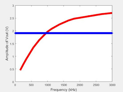 |
| Figure 9: High Pass filter circuit's data plotted with cutoff frequency |


Blog looks good. Curious if you guys had any trouble with matlab. There were a few incidents in which it took us a few tries to get the right code. Also, i was interested to see what values you obtained on your high and low pass filters. Overall, great job!
ReplyDeleteThe only problems we came across were at the end, when we had to calculate the cutoff frequency's at which to plot our line.
DeleteYour blog looks really good, it looks like you guys worked really hard on it this week. I had trouble using MATLAB because I am just not familiar with it, I didn't take EGR 200 I took CPS 180 instead! Your graphs look good, but wouldn't the high and low pass filter graphs be more of a straight line? Also if you took CPS 180, it's interesting to me how different java and MATLAB are, but similar at the same time. Maybe that is just me though! You guys did a great job on your blog.
ReplyDeletePersonally i took CPS 180, I believe Justin took EGR 200. But many other classes require you to use MATLAB in certain projects or assignments eventually you learn how to use it for basic things in engineering, because it has many applications to help people understand/solve problems.
Deletei think you made a good job solving these questions in matlab and i think it is hard a little bit for these who are not familier with matlab for me i have taken egr 200 so i know some information about matlab and how to deal with it.
ReplyDeleteThank you, if you took EGR 200 you probably know more about MATLAB than me.
Delete
ReplyDeleteGood blog organization. For Q#14 I think you have to show the critical point. Also, for high and low pass filters we have different graphs, maybe because we have different resister and capacitor. Otherwise, we have similar answers.
Good job