Blog Report Week 5

1. Functional check: Oscilloscope manual page 5. Perform the functional check (photo).

The displayed output on the oscilloscope, after the
functionality check is completed.

• Functionality Checks help ensure that the oscilloscope and its probes are working correctly. They should be done the first time it is used, as well as if the equipment has not been used in a while or is believed to be faulty. 

2. Perform manual probe compensation (Oscilloscope manual page 8) (Photo of overcompensation and proper compensation).

Photo 1: An "overcompensated" wave 

Photo 2: A corrected wave in
"proper compensation" 

• To adjust the probe, use a key to turn the screw inside of its hole until it is properly compensated on the oscilloscope's display.  

3. What does probe attenuation (1x vs. 10x) do (Oscilloscope manual page 9)?

• Some probes differ in their attenuation setting, you can tune these settings using the mechanical switch on the handle. Be sure that the oscilloscope's attenuation matches your probe's. By adjusting the attenuation, you're actually adjusting the impedance for a more accurate reading through you probes. Ensuring that your machines settings match those of your probe, you're allowing your machine to utilize its full bandwidth.

4. How do vertical and horizontal controls work? Why would you need it (Oscilloscope manual pages 34-35)?

• Vertical position adjusts the cursors on the oscilloscopes screen.
• Horizontal position of all channel and math waveform, its control varies with the time base setting.

• You can position the data from both channels, as you can choose to have them displayed separately or overlapping.

• The Scale controls allow the user to modify the display, so that the data can be enlarged or simplified for proper reading.

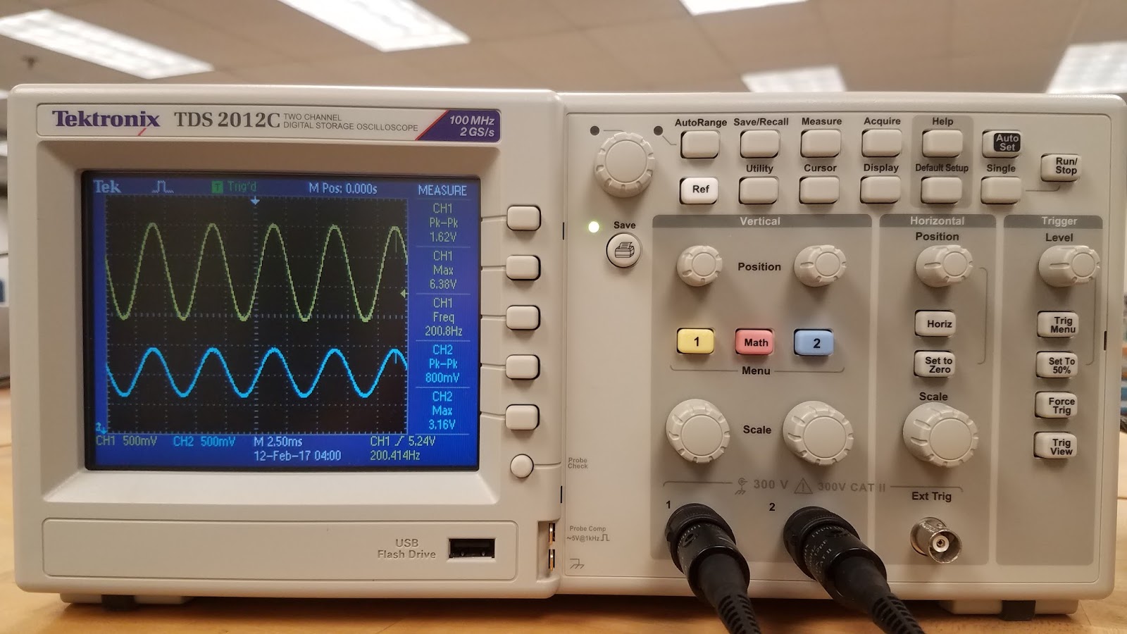
5. Generate a 1kHz, 0.5 Vpp around a DC 1V from the function generator (use the output connector). DO NOT USE oscilloscope probes for the function generator. There is a separate BNC cable for the function generator.

a.) Connect this to the oscilloscope and verify the input signal using the horizontal and vertical readings (photo).

The wave generated by the function generator values
displayed above.

• We were able to generate a 0.5V Pk-Pk signal using the function generator. We adjusted the adjusted the voltage output to be about 1V, the "Auto-Set" measurements in the picture above prove this.

b.) Figure out how to measure the signal properties using menu buttons on the scope.

• You can measure the signals properties by using the "Measure" button and adding the measurement tiles on the right side of the screen, in it you can access which channel and the type of measurement you want to monitor/record on the screen.

6. Connect function generator and oscilloscope probes switched (red to black, black to red). What happens? Why?

• The scope does not "Auto-Set" the display correctly, it looks like there is noise mixed in with the signal, since it's signal is continuous and does not look sinusoidal. This is happening because you're connecting the oscilloscope probe to the ground, which grounds the signal before the machine can read it.

7. After calibrating the second probe, implement the voltage divider circuit below (UPDATE! V2 should be 0.5 Vac and 2 Vdc). Measure the following voltages using the Oscilloscope and comment on your results:

a.) Va and Vb at the same time (Photo)

The Va and Vb Voltages measured from the above circuit

• The top (yellow) wave is Vb = CH1, while the bottom (blue) wave is Va = CH2. The values we used on the function generator were 1.01V for the AC (Our generator can't go below 1V) attempting to keep the [0.5 : 2]V as a ratio, we set the DC offset to 4V because of this. Also resistors R4 and R5 were not quite 1kΩ, they were actually about 1.183kΩ.

• Notice how Va has about double the Pk-Pk Voltage compared to Vb. So when Va has the amplitude of 801V, Vb  will have an amplitude around 400V. Because the Amplitude is half that of the Pk - Pk value.

b.) Voltage across R4.

Photo 1: Attempted way of measuring Voltage across R4.

Photo 2: Using "Math" Function to find Voltage difference

across R4.

• We attempted to directly measure the voltage across R4, but the didn't feel confident about the results because according to other blogs, you cant do this, so as a result we took the liberty to find an alternative way of measuring the voltage.
• The "Math" measurement is set to [Math = CH1 - CH2] on the oscilloscope. This allows it to display the difference between the Pk-Pk values. So [R4 = Vb - Va] = [1.66V- 840mV=820mV] (O-scope says 860mV).

8. For the same circuit above, measure Va and Vb using the handheld DMM both in AC and DC mode. What are your findings? Explain.

Recorded (AC & DC) RMS Voltages - Using Handheld DMM:

• In AC mode: Va = 2.81V, Vb = 561mV
• In DC mode: Va = 280mV, Vb = 561mV

• We found that the recorded DC voltage measurement for Vb doubles that of Va, what is odd is the difference between the AC voltages. From our understanding is voltage should be about the same across an entire circuit. The reason it is not is because if you attach the ground on the other side of a resistor you short the circuit, thus giving a different measurement than expected.

9. For the circuit below:

a.) Calculate R so given voltage values are satisfied. Explain your work (video)

Video explains how we calculated the resistance across R7

b.) Construct the circuit and measure the values with the DMM and oscilloscope (video). Hint: 1kΩ cannot be probed directly by the scope. But R6 and R7 are in series and it does not matter which one is connected to the function generator.

Video shows the measurement differences between DMM and oscilloscope.

10. Operational amplifier basics: Construct the following circuits using the pin diagram of the opamp. The half circle on top of the pin diagram corresponds to the notch on the integrated circuit (IC). Explanations of the pin numbers are below:

a.) Inverting amplifier: Rin = 1kΩ, Rf = 5kΩ (do not forget -10V and +10V). Apply 1 Vpp @ 1kHz. Observe input and output at the same time. What happens if you slowly increase the input voltage up to 5V? Explain your findings. (Video) 

Explaining inverting amplifier circuit, and changing its voltage

• When we re-scaled the horizontal wavelength, we noticed that the crest for CH1 took place at the same time as CH2 trough. When the input voltage is low around 1V, the output signal is a sine wave. However, this changed when we adjusted the input voltage up to about 5V, you can see that the output signal changed to more of a square step-like function wave. Pins 4 and 7 control the voltage output range on the LM741 (-10V to 10V is about 20V.) 

b.) Non-inverting amplifier: R1 = 1kΩ, R2 = 5kΩ (do not forget -10V and +10V). Apply 1 Vpp @ 1kHz. Observe input and output at the same time. What happens if you slowly increase the input voltage up to 5V? Explain your findings. (Video)

Non-inverting amplifier circuit, and what happens when we change its amplitude

• The signal on the non-inverting amplifier, just like its name says: is not inverted. When we increased the input voltage, the output signal was not affected. This could be because the output voltage reached its maximum while we increased the input voltage. Similar to the inverting amplifier, pins 4 and 7 control the voltage output range on the LM741 (-10V to 10V is about 20V.) 

Blog Report Week 4

1.

(Table and graph) Use the transistor by itself. The goal is to create the graph for IC (y-axis) versus VBE (x-axis). Connect base and collector. Use 10 KΩ potentiometer to generate the voltage. Use 5V but DO NOT EXCEED 1V for VBE. Make sure you have the required voltage value set before applying it to the base. Transistor might get really hot. Do not TOUCH THE TRANSISTOR! Make sure to get enough data points to graph. (Suggestion: measure for VBE = 0V, 0.5V, and 1V and fill the gaps if necessary by taking extra measurements). The circuit should look like the one below:

Data table 1: (Base/Emitter voltage)
and (Collector Current)

Graph 1: Data from table 1, modified to show the trend between Vbe and Ic.
Data #'s 7, 8 were removed to show exponential line.

• For the circuit schematic above, our class decided to discard the 10k Ω potentiometer and instead just adjust the amount voltage manually using the power supply. The recorded data above shows an exponential relationship between the collector and base currents, as soon as the Vbe voltage hits around 0.65 V, you can see its current begins to increase exponentially on a curve. We stopped recording data around 0.8 V so that we didn't burn the transistor out.

2. (Table and graph) Create the graph for IC (y axis) versus VCE (x axis). Vary VCE from 0 V to 5 V. Do this measurement for 3 different VBE values: 0V, 0.7V, and 0.8V. The circuit should look like below:

Data Table 2: Shows recorded measurement combinations of
Vbe, and Vce set to various voltages to show the different IC outputs. 

Graph 2: Shows the visual correlations of the data table above,
notice how the differing voltages create both linear and exponential lines.

3. (Table) Apply the following bias voltages and fill out the table. How is IC and IB related? Does your data support your theory?

Table 3: IC and IB are related because it is the currents flowing through the transistor, equation IE = IC + IB also proves their relationship

• IC and IB are related by beta (𝛃), 𝛃 = (IC / IB) our table above seems to be somewhat linear, thus we could say "yes, our data supports this theory." 

4. (Table) Explain photocell outputs with different light settings. Create a table for the light conditions and photocell resistance.

Table 4: Shows the amount of resistance is output due to
light conditions by the photocell

• A photocell outputs different resistances based on the amount of light it recieves. The more light it receives, the less amount of resistance is supplied to the circuit. Our data above supports this.

5. (Table) Apply voltage (0 to 5 V with 1 V steps) to DC motor directly and measure the current using the DMM.

Table 5: Shows the relationship between the voltage and
amount of current flowing through the DC motor.

6. Apply 2 V to the DC motor and measure the current. Repeat this by increasing the load on the DC motor. Slightly pinching the shaft would do the trick.

Table 6: Shows the amount of pressure applied to the
shaft of the motor, and the current being drawn by the motor.

7. (Video) Create the circuit below (same circuit from week 1). Explain the operation in detail.

                                           

8. Explain R4’s role by changing its value to a smaller and bigger resistors and observing the voltage and the current at the collector of the transistor.

Table 7: Shows that the more voltage and resistance in the
transistor, the more current will be in its collector

• The 47 Ω Resistor acts as a safety net for the transistor, almost like a fuse. It helps prevent any excess current that may come from the power supply. By raising the voltage it proves ohms law, that I = V/R, it starts increasing more

9. (Video) Create your own Rube Goldberg setup.